How To Make A Bar Chart Excel

How To Make A Bar Chart Excel - Bar charts are one of the most commonly used types of charts in Excel. They are a great way to visually represent data and make it easy to compare different values. In this post, we will show you how to create a bar chart in Excel with start time and duration.

Creating a bar chart in Excel

Step 1:

Open Microsoft Excel and select the data you want to use in your chart. In this example, we will be using start time and duration, so we have created a table with these columns:

Step 2:

Select the data you want to use for your chart. In this case, we are selecting the start time and duration columns.

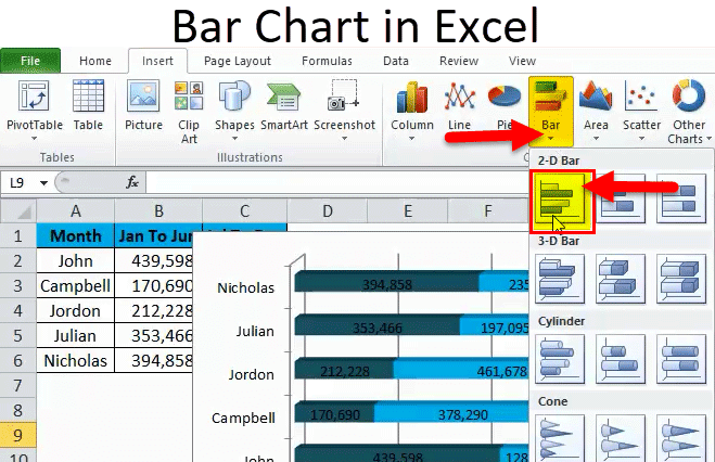
Step 3:

Click on the Insert tab on the Excel Ribbon and then click on the Bar Chart button. Choose the type of bar chart you want to create. In this example, we are selecting a stacked bar chart.

Step 4:

Edit the chart as needed. You can add labels, change the colors, and adjust the formatting to suit your needs.

Tips for creating a great bar chart in Excel

When creating a bar chart in Excel, there are a few things you can do to ensure it makes your data as clear and easy to understand as possible.

Tip 1: Choose the right type of bar chart. There are many types of bar charts in Excel, including stacked, grouped, and 3D. Each type has its own advantages and disadvantages, so choose the one that will best display your data.

Tip 2: Keep it simple. A cluttered chart will make it difficult to understand your data, so keep it simple and focused.

Tip 3: Use colors appropriately. Colors can help draw attention to important data points, but too many colors can be overwhelming. Stick to a few colors that work well together.

Tip 4: Label everything. Make sure your chart has clear labels for the x-axis, y-axis, and data points. This will help ensure that your audience understands the data you are trying to convey.

Ideas for using bar charts in Excel

Bar charts are a versatile tool that can be used in many different situations. Here are a few ideas for using bar charts in Excel:

Idea 1: Compare sales data. Use a bar chart to compare sales data for different products, regions, or time periods.

Idea 2: Track project progress. Use a bar chart to track the progress of a project, with each bar representing a task or milestone.

Idea 3: Analyze survey data. Use a bar chart to analyze survey data, with each bar representing the percentage of respondents who chose a particular answer.

How to customize a bar chart in Excel

Excel offers many options for customizing your bar chart. Here are a few ways to make your bar chart stand out:

Customize the colors: Change the colors of your bar chart by selecting the bars and going to the Format tab on the Ribbon. Select the color you want from the Fill Color dropdown.

Customize the labels: You can change the font, size, and style of your labels by selecting them and going to the Home tab on the Ribbon. You can also add data labels, axis labels, and titles to your chart from here.

Customize the chart type: If you want to change the type of chart you are using, you can do so by selecting the chart and going to the Design tab on the Ribbon. From here, you can choose from many different chart types, including line charts, pie charts, and scatter charts.

Customize the data: If you want to change the data that is displayed in your chart, you can do so by selecting the chart and clicking on the Select Data button on the Ribbon. From here, you can add or remove data series, change the order of the series, and more.

With these tips, ideas, and how-to steps, you should now be able to create a bar chart in Excel that effectively represents your data. Remember to keep it simple, label everything, and choose the right type of chart for your data. Happy charting!

View more articles about How To Make A Bar Chart Excel